Growth Processes
The Logistic and the Gompertz Function against a Sequence of Exponential Processes
H. Schneeberger
Institute of Statistics, University of Erlangen-Nürnberg, Germany
2013, 9th February
Introduction
Growth-Processes are well-known in natural sciences for a long time. For example Mendel's law (Mendel 1822-1884) in botany. Mitscherlich E.A. (1974-1956), an agronom, in 1909 found the dependence of crop-yield on the quantity of fertilizer. All these laws only described the ascending branch of the growth-process. The descending branch was of no interest - at that time.
Against that the economists already in the early decades of the 19th century sought for formulae, which could explain the ascending and the descending production-process. To simplify this problem, they took the cumulative production-data instead of the production-data. So they had to estimate the parameters of a mathematically simpler function. Parameter-estimation then was the problem with the actual mathematical and computer possibilities.
The solutions of two well-known differential-equations were suitable for this problem of approximating data with only positive trend: The logistic function and the Gompertz-function. It will be shown in this paper with the production-data of VW-beetle from 1950 to 2003, that for this application both hypotheses are unsuitable for describing the growth process, and why it is so: The restrictions of the two hypotheses are too grave. I suppose, that not many applications will fit to them in adequate way. As an alternative the direct way of estimating the growth of the production (not of the cumulative production) as a sequence of exponential processes is presented. With this method the number of parameters is much greater, the adaptation of data to hypothesis much more flexible. But nowadays estimation of many parameters is no problem with modern iterative mathematical methods and computers.
Preparatory remarks
As in the presented hypotheses Euler's e-function is of decisive importance, and the values of the variables X=year and Y=cumulated production (given in table 1) are very large, they must be transformed for computing variables. I choose
x=(X-1950)/10 and y=Y•10-6
To distinguish data Y resp. y from hypotheses, I use for the hypotheses the term ![]() (X) resp ŷ(x), as it is practised in statistics
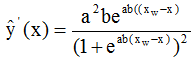
If the growth-function ŷ(x) of the cumulative production is computed, i.e. if the parameters of the function are estimated, then the growth-function of the production itself is also given as the differential of the logistic, resp. Gompertz function ŷ'(x)=... (see (1) and (7)). Therefore I will call dŷ/dx = ŷ'(x) also
(X) resp ŷ(x), as it is practised in statistics
If the growth-function ŷ(x) of the cumulative production is computed, i.e. if the parameters of the function are estimated, then the growth-function of the production itself is also given as the differential of the logistic, resp. Gompertz function ŷ'(x)=... (see (1) and (7)). Therefore I will call dŷ/dx = ŷ'(x) also ![]() (x) and d
(x) and d![]() /dX =
/dX = ![]() '(X) also
'(X) also ![]() (X). Then with
(X). Then with

we also have the production function ![]() '(X) = P(X) and the cumulative production-function
'(X) = P(X) and the cumulative production-function ![]() (X) in the original variable X (see figures 3, 4, 5, 6).
(X) in the original variable X (see figures 3, 4, 5, 6).
Methods
Logistic Function (Verhulst 1804-1849)
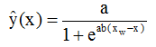
The logistic function is defined by the differential equation
![]() (1)
(1)
The solution is
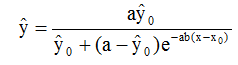 (2)
(2)
with the boundary-point (x0, ŷ0). Three parameters a, b, ŷ0 must be estimated.
In the literature the solution with y0 instead of ŷ0 = ŷ(x0) is to be found. This procedure reduces the number of parameters. But then the solution is another for every boundary point (x0, y0). This can yield very different solution-curves, especially for small y0-values at the beginning of the time-series. Against that the solution (2) yields the same curve for every boundary point (x0,ŷ0) with different values x0.
The three parameters are estimated with the method of Least-Squares of Gauß
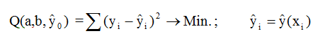 (3)
(3)
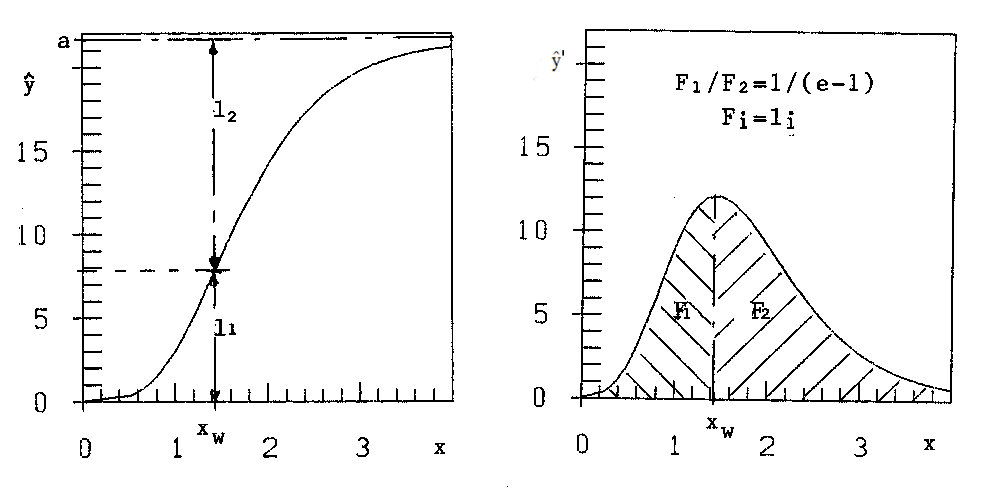
with the data-points (xi, yi) of table 1. The minimum is found with the iterative nonlinear Simplex Method of Nelder and Mead (Ref. 2). We get a=21.24, b=0.1099, ŷ0=3.347, with x0 = 1 . See figures 1a and 3a.
Figure 1a: Logistic curve ŷ(x)Figure 1b: ŷ'(x)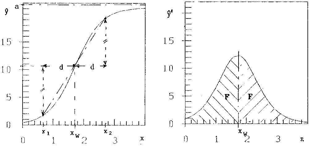
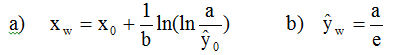
The well-known condition y''(x) = 0 for the point of inflection yields
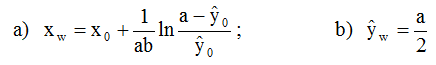 (4)
(4)
and herewith
 (5a)
(5a)
and
 (5b)
(5b)
Formulae (4) and (5) with d =xw - x1 = x2 - xw yield the restrictions
![]() (6a)
(6a)
and
![]() (6b)
(6b)
Together with condition (4b) these are a lot of restrictions, imposed on the growth-function ŷ(x). They mean the symmetry of the curve ŷ and inclination ŷ' to point (xw, ŷw ). See figure 1a. Still more evident are these restrictions in figure 1b, the representation of ŷ' = ![]() , of the production: The hypothesis of the logistic function assumes a production symmetric to x = xw
, of the production: The hypothesis of the logistic function assumes a production symmetric to x = xw
Gompertz-Function (Gompertz 1779-1861)
The Gompertz-function is defined by the differential equation
![]() (7)
(7)
with the solution
![]() (8)
(8)
with the boundary-point (x0, ŷ0 ) and the three parameters (a,b,ŷ0). The estimation of the parameters with the data of table 1 is done with the same procedure as with the logistic function. We get a = 21.66, b = 1.527, ŷ0 = 3.024, (x0 = 1). Figures 2a and 4a give the result.
Figure 2a: Gompertz curve ŷ(x) Figure 2b: ŷ'(x)
y''(x) = 0 gives for the point of inflection:
 (9)
(9)
and
 (10)
(10)
Condition (9b) is a serious restriction: 1/e or 36.8% of the production are on the left side, 63.2% on the right side of xw, i.e. of the maximum of the production-curve in figure 2b.
Sequence of exponential functions
Here, in this special application, the growth-process is explained by a series of four successive processes with data of the production, not of the cumulative production of VW-beetle in table 1.
Process I is an exponential process of type (see figure 5):
I ![]() (11)
(11)
as it is the case e.g. with nuclear fission. As (I) would result in an explosion, it turns into an exponential ascending process
II ![]() (12)
(12)
with horizontal asymptote, followed by an declining exponential process
III ![]() (13)
(13)
(see the symmetry to (II)), and at last turns into an exponential dying process
IV ![]() (14)
(14)
(see the symmetry to process (I)). The signs +/- of the parameters are chosen so, that the values of the parameters are positive.
Processes (I) and (IV) are well-known as starting and dying processes; (II) e.g. is known as Mendel's Law of Genetics. In agronomy Mitscherlich 1909 (Ref. 1) found "with an immense number of field experiments" formula (II) for the growth of crop-yield p in dependence on the quantity of fertilizer x. See also Ref. 4. The following overfertilization as a process of type (III) is a process, inverse to (II) - see Ref. 5. The stress-strain relationship (for small loading Hooke's linear law in mechanics) also is a sequence of processes (II) and (III), which is shown in Ref. 3 for concrete and steel. Especially in these technical applications with their homogenous material the agreement of data-points and hypothetical curve is very good. The values a of the two horizontal asymptotes of (II) and (III) are (practically) identical; curve (II) turns into curve (III) in a smooth way. It was an ideal material for a pilot-study.
The parameters for the four partial processes I-IV were again computed with the method of Least Squares, the minimum was found with Nelder and Mead (Ref. 2).
| Year of production | Number of production | Frequency in total |
| 1950 | 81.979 | 168.161 |
| 1951 | 93.709 | 261.870 |
| 1952 | 114.348 | 376.218 |
| 1953 | 151.323 | 527.541 |
| 1954 | 202.174 | 729.715 |
| 1955 | 279.986 | 1.009.701 |
| 1956 | 333.190 | 1.342.891 |
| 1957 | 380.561 | 1.723.452 |
| 1958 | 451.526 | 2.174.978 |
| 1959 | 575.406 | 2.750.384 |
| 1960 | 739.443 | 3.489.827 |
| 1961 | 827.850 | 4.317.677 |
| 1962 | 877.014 | 5.194.691 |
| 1963 | 838.488 | 6.033.179 |
| 1964 | 948.370 | 6.981.549 |
| 1965 | 1.090.863 | 8.072.412 |
| 1966 | 1.080.165 | 9.152.577 |
| 1967 | 925.787 | 10.078.364 |
| 1968 | 1.186.134 | 11.264.498 |
| 1969 | 1.219.314 | 12.483.812 |
| 1970 | 1.196.099 | 13.679.911 |
| 1971 | 1.291.612 | 14.971.523 |
| 1972 | 1.220.686 | 16.192.209 |
| 1973 | 1.206.018 | 17.398.227 |
| 1974 | 791.053 | 18.189.280 |
| 1975 | 441.116 | 18.630.396 |
| 1976 | 383.277 | 19.013.673 |
| 1977 | 258.634 | 19.272.307 |
| 1978 | 271.673 | 19.543.980 |
| 1979 | 263.340 | 19.807.320 |
| 1980 | 236.177 | 20.043.497 |
| 1981 | 157.505 | 20.201.002 |
| 1982 | 138.091 | 20.339.093 |
| 1983 | 119.745 | 20.458.838 |
| 1984 | 118.138 | 20.576.976 |
| 1985 | 86.189 | 20.663.165 |
| 1986 | 46.633 | 20.709.798 |
| 1987 | 17.166 | 20.726.964 |
| 1991 | 85.681 | 20.948.790 |
| 1992 | 86.613 | 21.035.403 |
| 1993 | 104.710 | 21.140.113 |
| 1994 | 95.600 | 21.235.713 |
| 1995 | 33.361 | 21.269.074 |
| 1996 | 39.722 | 21.308.796 |
| 1997 | 35.678 | 21.344.474 |
| 1998 | 36.492 | 21.380.966 |
| 1999 | 36.446 | 21.417.412 |
| 2000 | 41.260 | 21.458.672 |
| 2001 | 38.850 | 21.497.522 |
| 2002 | 24.407 | 21.521.929 |
| 2003 | 7.535 | 21.529.464 |
These data are given in the internet: www.ridemotion.com/379-VW; the data for 1988 are missing, the addition of date of 1989 to 1990 is faulty. So they were omitted.
Results and Discussion
Logistic Function
The parameters a, b, ŷ0 of formula (2) with data of table 1 are
a = 21.24, b = 0.1099, ŷ0 = 3.347 (x0 = 1 )
In figures 3a and 3b for the cumulative production-function (2) and for the production-function (1) data (as small squares) and solution-curves are given. I think, that in figure 3a the correspondence of data and curve is very good; that isn't the case for the production-curve in figure 3b. Beginning with about 1960 the curve drifts to the left of the data, caused by the postulated symmetry of the curve. The maximum per hypothesis (= per curve) is about at 1967, per data at 1971, the crash of the production between 1971 and 1975 from 1.29 to 0.44 million cars, i.e. down to 34%, is softened in the curve, also because of the forced symmetry. Of these discrepancies nothing can be seen in figure 3a at all! An entire wrong idea of correspondence of data and hypothesis is pretended.
Gompertz Function
The parameters of formula (8) are
a = 21.66, b = 1.527, ŷ0 = 3.024 (x0 = 1)
According to figure 4a one could perhaps state moderate agreement of hypothetical curve and data. Quite otherwise with figure 4b. Up to 1956 the curve is too low, from 1956 on it is too high and by far to the left. The maximum of the curve is at X=1964, while the maximum of the data is at X=1971! In short: data and figure 4b go their own way. The reason is the grave restriction: 36.8% of the production is before, 63.2% after the maximum of the curve. In reality it is rather vice versa.
Analysis of Logistic and especially Gompertz-function show, that the curves (3a) and (4a) for the cumulative data can give a totally wrong idea.
Sequence of exponential functions
Computation gives the parameters for processes I to IV in table 2. The trend-curves I to IV are given in figure 5.
The correspondence of data and curves for processes I and II is good. In the experiments of natural sciences (with steel and concrete (ref.3) and in agronomy (ref.5)) phase II short before the asymptote turns smoothly into the asymptote of phase III. Here the crash of the production is given as a break from phase II to phase III. In phase IV there is a great variability of the data. External effects may play a role, for example the so-called Mexico-beetle.
| x | x0 | a | b | ||
|---|---|---|---|---|---|
| I | 0 ≤ x ≤ 0.9 | 0 | 0.8303 | 2.16 | |
| II | 0.9 ≤ x ≤ 2.1 | 0.9 | 6.321 | 17.13 | 0.716 |
| III | 2.1 ≤ x ≤ 2.7 | 2.1 | 12.31 | 16.19 | 2.229 |
| IV | 2.7 ≤ x ≤ 5.3 | 2.7 | 3.075 | 1.093 |
Figure 3a: Cum. prod. curve with logistic hypothesis Figure 3b: Production curve with logistic hypothesis
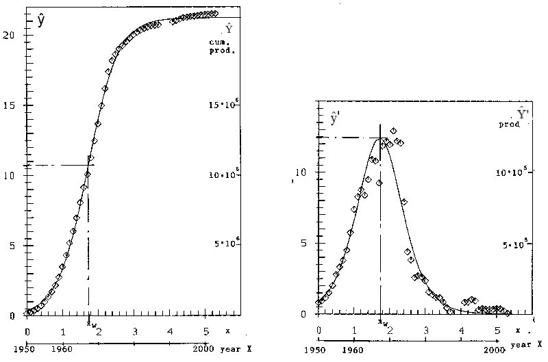
Figure 4a: Cum. prod. curve with Gompertz hypothesis Figure 4b: Production curve with Gompertz hypothesis
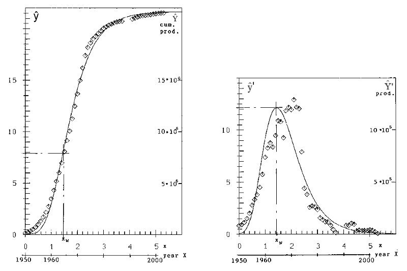
Figure 5: Production curve as a sequence of exponential functions
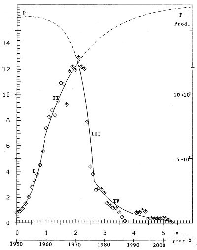
Figure 6: Comparison of production curves: Logistic function, Gompertz function,and a sequence of exponential functions
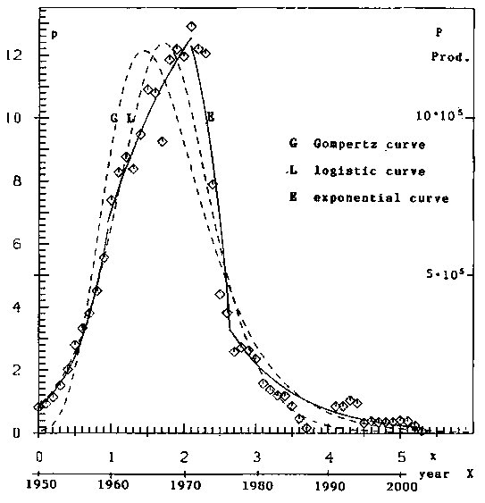
At last in figure 6 the growth-curves, found with the three hypotheses, are shown for direct comparison. The Gompertz-method gives by far the poorest result. This comes from the especially hard restriction of this hypothesis, that about 2/3 of the production is to the right of the maximum. The restriction 1/2 with the logistic method reduces the evil. With these data. The method with -in this example four- exponential functions and ten parameters easily outdoes the other methods with their three parameters. But estimation of many parameters is no problem nowadays: Mathematically and computerwise.
Epilogue
Do not only listen to the word,
and so deceive yourselves
James 1,22
In Luther's Übersetzung dieses Zitats aus dem Brief des Jakobus (Neues Testament)
Seid aber Täter des Worts
und nicht Hörer allein
wodurch Ihr euch selbst betrüget
References
- Mitscherlich E.A. (1909): Das Gesetz des Minimums und das Gesetz des abnehmenden Bodenertrags. Landwirtschaftliche Jahrbücher 38, 537-552
- Nelder J.R. and Mead R. (1965): A Simplex Method for the function minimization. The Computer Journal 7, 303-313
- Schneeberger H. (2005): Theory of the stress-strain relationship of concrete and steel. In: R.K. Dhir, M.D. Newlands and L.J. Csetenyi (eds.): Applications of Nanotechnology in Concrete Design. Proceedings of the Int. Conference at the University of Dundee, Scotland, UK, 105-112.
- Schneeberger H. (2009): Mitscherlich's Law: Sum of two exponential Processes. Conclusions. In internet: www.soil-statistic.de
- Schneeberger H. (2009): Overfertilization: An inverse Mitscherlich Process. In internet: www.soil-statistic.de